Experiment Tracking

Experiment Tracking#

Important

Experiment tracking requires ploomber-engine 0.0.11 or higher

ploomber-engine comes with a tracker that allows you to log variables, and plots without modifying your code. A common use case is for managing Machine Learning experiments. However, you can use it for any other computational experiments where you want to record input parameters, outputs, and analyze results.

Under the hood, it uses the SQliteTracker from our sklearn-evaluation package, this means that you will be able to query, and aggregate your experiments with SQL!

For this example, we’ll train several Machine Learning models and evaluate their performance.

Dependencies#

Before we run this example, we’ll need to install the required dependencies:

pip install ploomber-engine sklearn-evaluation jupytext --upgrade

Now, let’s download the sample script we’ll use, Jupyter notebooks (.ipynb) are also supported:

%%sh
curl -O https://raw.githubusercontent.com/ploomber/posts/master/experiment-tracking/fit.py

  % Total    % Received % Xferd  Average Speed   Time    Time     Time  Current

                                 Dload  Upload   Total   Spent    Left  Speed

  0     0    0     0    0     0      0      0 --:--:-- --:--:-- --:--:--     0
100  1718  100  1718    0     0  10628      0 --:--:-- --:--:-- --:--:-- 10670

Let’s create our grid of parameters, we’ll execute one experiment for each combination:

from ploomber_engine.tracking import track_execution
from sklearn.model_selection import ParameterGrid

grid = ParameterGrid(
    dict(
        n_estimators=[10, 15, 25, 50],
        model_type=["sklearn.ensemble.RandomForestClassifier"],
        max_depth=[5, 10, None],
        criterion=["gini", "entropy"],
    )
)

Let’s now execute the script multiple times, one per set of parameters, and store the results in the experiments.db SQLite database:

for idx, p in enumerate(grid):
    if (idx + 1) % 10 == 0:
        print(f"Executed {idx + 1}/{len(grid)} so far...")

    track_execution("fit.py", parameters=p, quiet=True, database="experiments.db")

Executed 10/24 so far...

Executed 20/24 so far...

If you prefer so, you can also execute scripts from the terminal:

python -m ploomber_engine.tracking fit.py \
    -p n_estimators=100,model_type=sklearn.ensemble.RandomForestClassifier,max_depth=10

No extra code needed#

If you look at the script’s source code, you’ll see that there are no extra imports or calls to log the experiments, it’s a vanilla Python script.

The tracker runs the code, and it logs everything that meets any of the following conditions:

1. A line that contains a variable name by itself

accuracy = accuracy_score(y_test, y_pred)
accuracy

2. A line that calls a function with no variable assignment

plot.confusion_matrix(y_test, y_pred)

Note that logs happen in groups (not line-by-line). A group is defined as a contiguous set of lines delimited with line breaks:

# first group
accuracy = accuracy_score(y_test, y_pred)
accuracy

# second group
plot.confusion_matrix(y_test, y_pred)

Regular Python objects are supported (numbers, strings, lists, dictionaries), and any object with a rich representation will also work (e.g., matplotlib charts).

Querying experiments with SQL#

After finishing executing the experiments, we can initialize our database (experiments.db) and explore the results:

from sklearn_evaluation import SQLiteTracker

tracker = SQLiteTracker("experiments.db")

Since this is a SQLite database, we can use SQL to query our data using the .query method. By default, we get a pandas.DataFrame:

df = tracker.query(
    """
SELECT *
FROM experiments
LIMIT 5
"""
)

type(df)

pandas.core.frame.DataFrame

df.head(3)

	created	parameters	comment
uuid
121fa9ab	2024-02-28 13:49:25	{"criterion": "gini", "max_depth": 5, "model_t...	None
8ee4f3b1	2024-02-28 13:49:26	{"criterion": "gini", "max_depth": 5, "model_t...	None
64364481	2024-02-28 13:49:26	{"criterion": "gini", "max_depth": 5, "model_t...	None

The logged parameters are stored in the parameters column. This column is a JSON object, and we can inspect the JSON keys with the .get_parameters_keys() method:

tracker.get_parameters_keys()

['accuracy',
 'classification_report',
 'confusion_matrix',
 'criterion',
 'f1',
 'max_depth',
 'model_type',
 'n_estimators',
 'precision',
 'precision_recall',
 'recall']

To get a sample query, we can use the .get_sample_query() method:

print(tracker.get_sample_query())

SELECT
    uuid,
    json_extract(parameters, '$.accuracy') as accuracy,
    json_extract(parameters, '$.classification_report') as classification_report,
    json_extract(parameters, '$.confusion_matrix') as confusion_matrix,
    json_extract(parameters, '$.criterion') as criterion,
    json_extract(parameters, '$.f1') as f1,
    json_extract(parameters, '$.max_depth') as max_depth,
    json_extract(parameters, '$.model_type') as model_type,
    json_extract(parameters, '$.n_estimators') as n_estimators,
    json_extract(parameters, '$.precision') as precision,
    json_extract(parameters, '$.precision_recall') as precision_recall,
    json_extract(parameters, '$.recall') as recall
    FROM experiments
LIMIT 10

Let’s perform a simple query that extracts our metrics, sorts by F1 score, and returns the top three experiments:

tracker.query(
    """
SELECT
    uuid,
    json_extract(parameters, '$.f1') as f1,
    json_extract(parameters, '$.accuracy') as accuracy,
    json_extract(parameters, '$.criterion') as criterion,
    json_extract(parameters, '$.n_estimators') as n_estimators,
    json_extract(parameters, '$.precision') as precision,
    json_extract(parameters, '$.recall') as recall
FROM experiments
ORDER BY f1 DESC
LIMIT 3
""",
    as_frame=False,
    render_plots=False,
)

uuid	f1	accuracy	criterion	n_estimators	precision	recall
6f138c8a	0.799659	0.786061	entropy	50	0.748672	0.858100
b6e2de28	0.799646	0.793939	entropy	50	0.774543	0.826431
32dd8e9d	0.795408	0.789394	gini	25	0.769801	0.822777

Rendering plots#

Plots are essential for evaluating our analysis, and the experiment tracker can log them automatically. So let’s pull the top 2 experiments (by F1 score) and get their confusion matrices, precision-recall curves, and classification reports. Note that we passed as_frame=False and render_plots=True to the .query method:

top_two = tracker.query(
    """
SELECT
    uuid,
    json_extract(parameters, '$.f1') as f1,
    json_extract(parameters, '$.confusion_matrix') as confusion_matrix,
    json_extract(parameters, '$.precision_recall') as precision_recall,
    json_extract(parameters, '$.classification_report') as classification_report
FROM experiments
ORDER BY f1 DESC
LIMIT 2
""",
    as_frame=False,
    render_plots=True,
)

top_two

uuid	f1	confusion_matrix	precision_recall	classification_report
6f138c8a	0.799659
b6e2de28	0.799646

Comparing plots#

If you want to zoom into a couple of experiment plots, you can select one and create a tab view. First, let’s retrieve the confusion matrices from the top 2 experiments:

top_two.get("confusion_matrix")

The buttons in the top bar allow us to switch between the two plots of the selected experiments. We can do the same with the precision-recall curve:

top_two.get("precision_recall")

Note that the tabs will take the value of the first column in our query (in our case, the experiment ID). So let’s switch them to show the F1 score via the index_by argument:

top_two.get("classification_report", index_by="f1")

Aggregation and plotting#

Using SQL gives us power and flexibility to answer sophisticated questions about our experiments.

For example, let’s say we want to know the effect of the number of trees (n_estimators) on our metrics. We can quickly write a SQL that aggregates by n_estimators and computes the mean of all our metrics; then, we can plot the values.

First, let’s run the query. Note that we’re passing as_frame=True so we get a pandas.DataFrame we can manipulate:

df = tracker.query(
    """
SELECT
    json_extract(parameters, '$.n_estimators') as n_estimators,
    AVG(json_extract(parameters, '$.accuracy')) as accuracy,
    AVG(json_extract(parameters, '$.precision')) as precision,
    AVG(json_extract(parameters, '$.recall')) as recall,
    AVG(json_extract(parameters, '$.f1')) as f1
FROM experiments
GROUP BY n_estimators
""",
    as_frame=True,
).set_index("n_estimators")

df

	accuracy	precision	recall	f1
n_estimators
10	0.751667	0.728144	0.808973	0.764190
15	0.757172	0.727507	0.822067	0.771398
25	0.767525	0.735006	0.835972	0.781861
50	0.768485	0.735331	0.839931	0.783535

Now, let’s create the plot:

import matplotlib.pyplot as plt

fig, ax = plt.subplots()

for metric in ["accuracy", "f1", "recall", "precision"]:
    df[metric].plot(ax=ax, marker="o", style="--")

ax.legend()
ax.grid()
ax.set_title("Effect of increasing n_estimators")
ax.set_ylabel("Metric")
_ = ax.set_xticks(df.index)

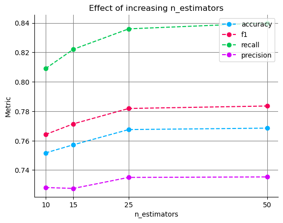
../_images/76fc9f3851bb23e75543c89e597ac4af0b253a798da50ae38a76e869cfef1a40.png

We can see that increasing n_estimators drives our metrics up; however, after 25 estimators, the improvements get increasingly small. Considering that a larger number of n_estimators will increase the runtime of each experiment, we can use this plot to inform our following experiments, cap n_estimators, and focus on other parameters.

If you need more details on how to work with the SQLiteTracker, you cna jump directly to the full example in the documentation.